This was originally written as a note on how to build tables with complex values i.e. values other than those supported in pivot tables.It focused on using range names and countif[s]/sumif[s]. One of the side effects was to document the use of range arrays and functional filtering. i.e. specifying an array within a cell and filtering the values down to one. This later piece of functionality has caused me to return to this page more frequently than the table construction. I have amended the tags and inserted this paragraph as finding it proved harder than I wanted.
I was recently doing some analytic work using spreadsheets; I was using pivot tables because they’re quick to make, but also felt that the median average best represented my data sets. The Excel pivot table does not support the median as a calculated value.
To solve this problem I used boolean functions and named arrays. This technique can also be used to filter arrays. Once again here is my data.

Figure 1: Data Set
I name the columns in the data array, in this case, I have named the names ‘names3’ and the values ‘values3’ because they are on the third tab called ‘Booleans + FDs’ in the sample spreadsheet.
Functions such as MAX & MEDIAN will take boolean functions instead of an array value and evaluate the boolean function as a filter. These functions must be saved as array functions i.e. by using the [Ctrl][SHIFT] & [ENTER] keys.
{=MAX(IF(names3=J9,values3))}
where J9 contains a string which exists within the names column of the data set.
{=MEDIAN(IF(names3=J9,values3))}
does the same for using the Median function and the picture below shows the effect of using these functions. This is common Excel *IF syntax. The first argument specifies a condition where a 1-dimensional array i.e. a column is specified by name and evaluated, in this case, against a value. In the example above the value is specified as the contents of a cell, an explicit string declaration also works. The second IF function argument is an array of values, and the corresponding value by position in the array is included in the results set. (I have not tested the effect of having different sized arrays.) This IF function replaces the array in the outer function, in the case of our examples above, MAX & MEDIAN.
Technically, this is not a pivot table; the names, Alfie, Bill … etc, would need to be on the horizontal axis for this to be true, but the Excel techniques will work in that case as well. The sample spreadsheet now includes a pivot table example. (DFL 7 Feb 2011.)
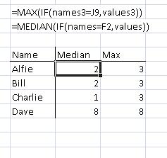
Figure 2: Filtered Median and Max
This technique also works for frequency distributions. In order to build a frequency distribution, one needs to define the class buckets. I am going to build f(Dave) which has the set values (4,8,8) . My FD maximum is going to be 10, and I am going to have an interval of 1. My buckets are thus (0,1,2,…,10). There are eleven elements. In the example file, I name the bucket array , “buckets”. In order to create an FD using the FREQUENCY function one must select an empty array of the same size as the bucket array and then insert the following function,
{=FREQUENCY(IF(names3=F1,values3),buckets)}
The {} means that this is an array function, and must be saved using [Ctrl][SHIFT] & [ENTER] keys. The frequency distribution appears below.

Figure 3: Filtered Frequency Distribution
In case you missed the referene above, I have updated the the sample spreadsheet which is available over http to include the examples in this blog article. The example sheet now includes a pivot table example. (DFL 7 Feb 2011.)
I discovered the boolean values with the help of my Citihub colleague, Tim Reczek. Thanks Tim. He also pointed me at these three links, which I found useful while solving this problem, these sites also have answers to a bunch of other problems.
- http://www.cpearson.com/Excel/ArrayFormulas.aspx
- http://www.mrexcel.com/articles/CSE-array-formulas-excel.php
- http://www.ozgrid.com/Excel/arrays.htm
Edited: Dave 7th Feb 2011
I edited this post on the 7th Feb 2011. I have amended the example spreadsheet to include a pivot example as the title states. I have improved the explanation of the use of named arrays and the boolean declarations, or at least made it longer. I have included three links that I found useful when doing the work that inspired this article. (I have also reduced the size of Fig. 1, which I hope improves readability.)
I have edited this post and amended the tag list to emphasise the content related to array filtering.